
Graph Data Structure And Algorithms
A Graph consists of a finite set of vertices(or nodes) and set of Edges which connect a pair of nodes.
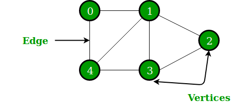 In the above Graph, the set of vertices V = {0,1,2,3,4} and the set of edges E = {01, 12, 23, 34, 04, 14, 13}.
Graphs are used to solve many real-life problems. Graphs are used to represent networks. The networks may include paths in a city or telephone network or circuit network. Graphs are also used in social networks like linkedIn, Facebook. For example, in Facebook, each person is represented with a vertex(or node). Each node is a structure and contains information like person id, name, gender, locale etc.
In the above Graph, the set of vertices V = {0,1,2,3,4} and the set of edges E = {01, 12, 23, 34, 04, 14, 13}.
Graphs are used to solve many real-life problems. Graphs are used to represent networks. The networks may include paths in a city or telephone network or circuit network. Graphs are also used in social networks like linkedIn, Facebook. For example, in Facebook, each person is represented with a vertex(or node). Each node is a structure and contains information like person id, name, gender, locale etc.
A Graph consists of a finite set of vertices(or nodes) and set of Edges which connect a pair of nodes.
Graph Data Structure
Mathematical graphs can be represented in data structure. We can represent a graph using an array of vertices and a two-dimensional array of edges. Before we proceed further, let's familiarize ourselves with some important terms −
-
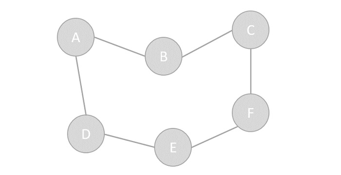
Vertex − Each node of the graph is represented as a vertex. In the following example, the labeled circle represents vertices. Thus, A to G are vertices. We can represent them using an array as shown in the following image. Here A can be identified by index 0. B can be identified using index 1 and so on.
-
Edge − Edge represents a path between two vertices or a line between two vertices. In the following example, the lines from A to B, B to C, and so on represents edges. We can use a two-dimensional array to represent an array as shown in the following image. Here AB can be represented as 1 at row 0, column 1, BC as 1 at row 1, column 2 and so on, keeping other combinations as 0.
-
Adjacency − Two node or vertices are adjacent if they are connected to each other through an edge. In the following example, B is adjacent to A, C is adjacent to B, and so on.
-
Path − Path represents a sequence of edges between the two vertices. In the following example, ABCD represents a path from A to D.
Mathematical graphs can be represented in data structure. We can represent a graph using an array of vertices and a two-dimensional array of edges. Before we proceed further, let's familiarize ourselves with some important terms −
- Vertex − Each node of the graph is represented as a vertex. In the following example, the labeled circle represents vertices. Thus, A to G are vertices. We can represent them using an array as shown in the following image. Here A can be identified by index 0. B can be identified using index 1 and so on.
- Edge − Edge represents a path between two vertices or a line between two vertices. In the following example, the lines from A to B, B to C, and so on represents edges. We can use a two-dimensional array to represent an array as shown in the following image. Here AB can be represented as 1 at row 0, column 1, BC as 1 at row 1, column 2 and so on, keeping other combinations as 0.
- Adjacency − Two node or vertices are adjacent if they are connected to each other through an edge. In the following example, B is adjacent to A, C is adjacent to B, and so on.
- Path − Path represents a sequence of edges between the two vertices. In the following example, ABCD represents a path from A to D.
Basic Operations
Following are basic primary operations of a Graph −
-
Add Vertex − Adds a vertex to the graph.
-
Add Edge − Adds an edge between the two vertices of the graph.
-
Display Vertex − Displays a vertex of the graph.
Following are basic primary operations of a Graph −
- Add Vertex − Adds a vertex to the graph.
- Add Edge − Adds an edge between the two vertices of the graph.
- Display Vertex − Displays a vertex of the graph.
Graph Terminology
We use the following terms in graph data structure...
We use the following terms in graph data structure...
Vertex
Individual data element of a graph is called as Vertex. Vertex is also known as node. In above example graph, A, B, C, D & E are known as vertices.
Edge
An edge is a connecting link between two vertices. Edge is also known as Arc. An edge is represented as (startingVertex, endingVertex). For example, in above graph the link between vertices A and B is represented as (A,B). In above example graph, there are 7 edges (i.e., (A,B), (A,C), (A,D), (B,D), (B,E), (C,D), (D,E)).
Edges are three types.
- Undirected Edge - An undirected egde is a bidirectional edge. If there is undirected edge between vertices A and B then edge (A , B) is equal to edge (B , A).
- Directed Edge - A directed egde is a unidirectional edge. If there is directed edge between vertices A and B then edge (A , B) is not equal to edge (B , A).
- Weighted Edge - A weighted egde is a edge with value (cost) on it.
Edges are three types.
Undirected Graph
A graph with only undirected edges is said to be undirected graph.
Directed Graph
A graph with only directed edges is said to be directed graph.
Mixed Graph
A graph with both undirected and directed edges is said to be mixed graph.
End vertices or Endpoints
The two vertices joined by edge are called end vertices (or endpoints) of that edge.
Origin
If a edge is directed, its first endpoint is said to be the origin of it.
Destination
If a edge is directed, its first endpoint is said to be the origin of it and the other endpoint is said to be the destination of that edge.
Adjacent
If there is an edge between vertices A and B then both A and B are said to be adjacent. In other words, vertices A and B are said to be adjacent if there is an edge between them.
Incident
Edge is said to be incident on a vertex if the vertex is one of the endpoints of that edge.
Outgoing Edge
A directed edge is said to be outgoing edge on its origin vertex.
Incoming Edge
A directed edge is said to be incoming edge on its destination vertex.
Degree
Total number of edges connected to a vertex is said to be degree of that vertex.
Indegree
Total number of incoming edges connected to a vertex is said to be indegree of that vertex.
Outdegree
Total number of outgoing edges connected to a vertex is said to be outdegree of that vertex.
Parallel edges or Multiple edges
If there are two undirected edges with same end vertices and two directed edges with same origin and destination, such edges are called parallel edges or multiple edges.
Self-loop
Edge (undirected or directed) is a self-loop if its two endpoints coincide with each other.
Simple Graph
A graph is said to be simple if there are no parallel and self-loop edges.
Path
A path is a sequence of alternate vertices and edges that starts at a vertex and ends at other vertex such that each edge is incident to its predecessor and successor vertex.
Graph Traversal - DFS
Graph traversal is a technique used for a searching vertex in a graph. The graph traversal is also
used to decide the order of vertices is visited in the search process. A graph traversal finds the
edges to be used in the search process without creating loops. That means using graph traversal
we visit all the vertices of the graph without getting into looping path.
There are two graph traversal techniques and they are as follows...
- DFS (Depth First Search)
- BFS (Breadth First Search)
Graph traversal is a technique used for a searching vertex in a graph. The graph traversal is also
used to decide the order of vertices is visited in the search process. A graph traversal finds the
edges to be used in the search process without creating loops. That means using graph traversal
we visit all the vertices of the graph without getting into looping path.
There are two graph traversal techniques and they are as follows...
There are two graph traversal techniques and they are as follows...
- DFS (Depth First Search)
- BFS (Breadth First Search)
DFS (Depth First Search)
DFS traversal of a graph produces a spanning tree as final result. Spanning Tree is a graph without loops.
We use Stack data structure with maximum size of total number of vertices in the graph to implement DFS traversal.
We use the following steps to implement DFS traversal...
- Step 1 - Define a Stack of size total number of vertices in the graph.
- Step 2 - Select any vertex as starting point for traversal. Visit that vertex and push it on to the Stack
- Step 3 - Visit any one of the non-visited adjacent vertices of a vertex which is at the top of stack and push it on to the stack.
- Step 4 - Repeat step 3 until there is no new vertex to be visited from the vertex which is at the top of the stack.
- Step 5 - When there is no new vertex to visit then use back tracking and pop one vertex from the stack.
- Step 6 - Repeat steps 3, 4 and 5 until stack becomes Empty.
- Step 7 - When stack becomes Empty, then produce final spanning tree by removing unused edges from the graph
DFS traversal of a graph produces a spanning tree as final result. Spanning Tree is a graph without loops.
We use Stack data structure with maximum size of total number of vertices in the graph to implement DFS traversal.
We use the following steps to implement DFS traversal...
We use the following steps to implement DFS traversal...
- Step 1 - Define a Stack of size total number of vertices in the graph.
- Step 2 - Select any vertex as starting point for traversal. Visit that vertex and push it on to the Stack
- Step 3 - Visit any one of the non-visited adjacent vertices of a vertex which is at the top of stack and push it on to the stack.
- Step 4 - Repeat step 3 until there is no new vertex to be visited from the vertex which is at the top of the stack.
- Step 5 - When there is no new vertex to visit then use back tracking and pop one vertex from the stack.
- Step 6 - Repeat steps 3, 4 and 5 until stack becomes Empty.
- Step 7 - When stack becomes Empty, then produce final spanning tree by removing unused edges from the graph
Graph Traversal - BFS
Graph traversal is a technique used for searching a vertex in a graph. The graph traversal is also used to
decide the order of vertices is visited in the search process. A graph traversal finds the edges to be
used in the search process without creating loops. That means using graph traversal we visit all the vertices
of the graph without getting into looping path.
There are two graph traversal techniques and they are as follows...
- DFS (Depth First Search)
- BFS (Breadth First Search)
Graph traversal is a technique used for searching a vertex in a graph. The graph traversal is also used to
decide the order of vertices is visited in the search process. A graph traversal finds the edges to be
used in the search process without creating loops. That means using graph traversal we visit all the vertices
of the graph without getting into looping path.
There are two graph traversal techniques and they are as follows...
There are two graph traversal techniques and they are as follows...
- DFS (Depth First Search)
- BFS (Breadth First Search)
BFS (Breadth First Search)
BFS traversal of a graph produces a spanning tree as final result.
Spanning Tree is a graph without loops.
We use Queue data structure with maximum size of total number
of vertices in the graph to implement BFS traversal.
We use the following steps to implement BFS traversal...
- Step 1 - Define a Queue of size total number of vertices in the graph.
- Step 2 - Select any vertex as starting point for traversal.
- Visit that vertex and insert it into the Queue.
- Step 3 - Visit all the non-visited adjacent vertices of the vertex
- which is at front of the Queue and insert them into the Queue.
- Step 4 - When there is no new vertex to be visited from the
- vertex which is at front of the Queue then delete that vertex.
- Step 5 - Repeat steps 3 and 4 until queue becomes empty.
- Step 6 - When queue becomes empty, then produce final
- spanning tree by removing unused edges from the graph
Graph and its representations
BFS traversal of a graph produces a spanning tree as final result.
Spanning Tree is a graph without loops.
We use Queue data structure with maximum size of total number
of vertices in the graph to implement BFS traversal.
We use the following steps to implement BFS traversal...
We use the following steps to implement BFS traversal...
- Step 1 - Define a Queue of size total number of vertices in the graph.
- Step 2 - Select any vertex as starting point for traversal.
- Visit that vertex and insert it into the Queue.
- Step 3 - Visit all the non-visited adjacent vertices of the vertex
- which is at front of the Queue and insert them into the Queue.
- Step 4 - When there is no new vertex to be visited from the
- vertex which is at front of the Queue then delete that vertex.
- Step 5 - Repeat steps 3 and 4 until queue becomes empty.
- Step 6 - When queue becomes empty, then produce final
- spanning tree by removing unused edges from the graph
Graph is a data structure that consists of following two components:
1. A finite set of vertices also called as nodes.
2. A finite set of ordered pair of the form (u, v) called as edge. The pair is ordered because (u, v) is not same as (v, u) in case of a directed graph(di-graph). The pair of the form (u, v) indicates that there is an edge from vertex u to vertex v. The edges may contain weight/value/cost.
Graphs are used to represent many real-life applications: Graphs are used to represent networks. The networks may include paths in a city or telephone network or circuit network. Graphs are also used in social networks like linkedIn, Facebook. For example, in Facebook, each person is represented with a vertex(or node). Each node is a structure and contains information like person id, name, gender and locale. See this for more applications of graph.
Following is an example of an undirected graph with 5 vertices.
 Following two are the most commonly used representations of a graph.
1. Adjacency Matrix
2. Adjacency List
There are other representations also like, Incidence Matrix and Incidence List. The choice of the graph representation is situation specific. It totally depends on the type of operations to be performed and ease of use.
Adjacency Matrix:
Adjacency Matrix is a 2D array of size V x V where V is the number of vertices in a graph. Let the 2D array be adj[][], a slot adj[i][j] = 1 indicates that there is an edge from vertex i to vertex j. Adjacency matrix for undirected graph is always symmetric. Adjacency Matrix is also used to represent weighted graphs. If adj[i][j] = w, then there is an edge from vertex i to vertex j with weight w.
We can represent a graph using Adjacency matrix. The given matrix is an adjacency matrix. It is a binary, square matrix and from ith row to jth column, if there is an edge, that place is marked as 1. When we will try to represent an undirected graph using adjacency matrix, the matrix will be symmetric.
The adjacency matrix for the above example graph is:
 Pros: Representation is easier to implement and follow. Removing an edge takes O(1) time. Queries like whether there is an edge from vertex ‘u’ to vertex ‘v’ are efficient and can be done O(1).
Cons: Consumes more space O(V^2). Even if the graph is sparse(contains less number of edges), it consumes the same space. Adding a vertex is O(V^2) time.
Pros: Representation is easier to implement and follow. Removing an edge takes O(1) time. Queries like whether there is an edge from vertex ‘u’ to vertex ‘v’ are efficient and can be done O(1).
Cons: Consumes more space O(V^2). Even if the graph is sparse(contains less number of edges), it consumes the same space. Adding a vertex is O(V^2) time.
Please see this for a sample Python implementation of adjacency matrix.
Adjacency List:
An array of lists is used. Size of the array is equal to the number of vertices. Let the array be array[]. An entry array[i] represents the list of vertices adjacent to the ith vertex. This representation can also be used to represent a weighted graph. The weights of edges can be represented as lists of pairs. Following is adjacency list representation of the above graph.
This is another type of graph representation. It is called the adjacency list. This representation is based on Linked Lists. In this approach, each Node is holding a list of Nodes, which are Directly connected with that vertices. At the end of list, each node is connected with the null values to tell that it is the end node of that list.

Graph is a data structure that consists of following two components:
1. A finite set of vertices also called as nodes.
2. A finite set of ordered pair of the form (u, v) called as edge. The pair is ordered because (u, v) is not same as (v, u) in case of a directed graph(di-graph). The pair of the form (u, v) indicates that there is an edge from vertex u to vertex v. The edges may contain weight/value/cost.
Graphs are used to represent many real-life applications: Graphs are used to represent networks. The networks may include paths in a city or telephone network or circuit network. Graphs are also used in social networks like linkedIn, Facebook. For example, in Facebook, each person is represented with a vertex(or node). Each node is a structure and contains information like person id, name, gender and locale. See this for more applications of graph.
Following is an example of an undirected graph with 5 vertices.
Following two are the most commonly used representations of a graph.
1. Adjacency Matrix
2. Adjacency List
There are other representations also like, Incidence Matrix and Incidence List. The choice of the graph representation is situation specific. It totally depends on the type of operations to be performed and ease of use.
1. Adjacency Matrix
2. Adjacency List
There are other representations also like, Incidence Matrix and Incidence List. The choice of the graph representation is situation specific. It totally depends on the type of operations to be performed and ease of use.
Adjacency Matrix:
Adjacency Matrix is a 2D array of size V x V where V is the number of vertices in a graph. Let the 2D array be adj[][], a slot adj[i][j] = 1 indicates that there is an edge from vertex i to vertex j. Adjacency matrix for undirected graph is always symmetric. Adjacency Matrix is also used to represent weighted graphs. If adj[i][j] = w, then there is an edge from vertex i to vertex j with weight w.
Adjacency Matrix is a 2D array of size V x V where V is the number of vertices in a graph. Let the 2D array be adj[][], a slot adj[i][j] = 1 indicates that there is an edge from vertex i to vertex j. Adjacency matrix for undirected graph is always symmetric. Adjacency Matrix is also used to represent weighted graphs. If adj[i][j] = w, then there is an edge from vertex i to vertex j with weight w.
We can represent a graph using Adjacency matrix. The given matrix is an adjacency matrix. It is a binary, square matrix and from ith row to jth column, if there is an edge, that place is marked as 1. When we will try to represent an undirected graph using adjacency matrix, the matrix will be symmetric.
The adjacency matrix for the above example graph is:
Pros: Representation is easier to implement and follow. Removing an edge takes O(1) time. Queries like whether there is an edge from vertex ‘u’ to vertex ‘v’ are efficient and can be done O(1).
Cons: Consumes more space O(V^2). Even if the graph is sparse(contains less number of edges), it consumes the same space. Adding a vertex is O(V^2) time.
Please see this for a sample Python implementation of adjacency matrix.
Please see this for a sample Python implementation of adjacency matrix.
Adjacency List:
An array of lists is used. Size of the array is equal to the number of vertices. Let the array be array[]. An entry array[i] represents the list of vertices adjacent to the ith vertex. This representation can also be used to represent a weighted graph. The weights of edges can be represented as lists of pairs. Following is adjacency list representation of the above graph.
This is another type of graph representation. It is called the adjacency list. This representation is based on Linked Lists. In this approach, each Node is holding a list of Nodes, which are Directly connected with that vertices. At the end of list, each node is connected with the null values to tell that it is the end node of that list.
No comments:
Post a Comment