
Keys in DBMS-
Different Types Of Keys in DBMS-
There are following 10 important keys in DBMS-

- Super key
- Candidate key
- Primary key
- Alternate key
- Foreign key
- Partial key
- Composite key
- Unique key
- Surrogate key
- Secondary key
1. Super Key-
- A super key is a set of attributes that can identify each tuple uniquely in the given relation.
- A super key is not restricted to have any specific number of attributes.
- Thus, a super key may consist of any number of attributes.
- A super key is a set of attributes that can identify each tuple uniquely in the given relation.
- A super key is not restricted to have any specific number of attributes.
- Thus, a super key may consist of any number of attributes.
Example-
Consider the following Student schema-
Student ( roll , name , sex , age , address , class , section )
Given below are the examples of super keys since each set can uniquely identify each student in the Student table-
- ( roll , name , sex , age , address , class , section )
- ( class , section , roll )
- (class , section , roll , sex )
- ( name , address )
NOTE-
All the attributes in a super key are definitely sufficient to identify each tuple uniquely in the given relation but all of them may not be necessary.
All the attributes in a super key are definitely sufficient to identify each tuple uniquely in the given relation but all of them may not be necessary.
2. Candidate Key- A set of minimal attribute(s) that can identify each tuple uniquely in the given relation is called as a candidate key.
Example-
Consider the following Student schema-
Student ( roll , name , sex , age , address , class , section )
Given below are the examples of candidate keys since each set consists of minimal attributes required to identify each student uniquely in the Student table-
- ( class , section , roll )
- ( name , address )
NOTES-
- All the attributes in a candidate key are sufficient as well as necessary to identify each tuple uniquely.
- Removing any attribute from the candidate key fails in identifying each tuple uniquely.
- The value of candidate key must always be unique.
- The value of candidate key can never be NULL.
- It is possible to have multiple candidate keys in a relation.
- Those attributes which appears in some candidate key are called as prime attributes.
3. Primary Key-
A primary key is a candidate key that the database designer selects while designing the database.
OR
Candidate key that the database designer implements is called as a primary key.
NOTES-
- The value of primary key can never be NULL.
- The value of primary key must always be unique.
- The values of primary key can never be changed i.e. no updation is possible.
- The value of primary key must be assigned when inserting a record.
- A relation is allowed to have only one primary key.
Remember-

4. Alternate Key-
Candidate keys that are left unimplemented or unused after implementing the primary key are called as alternate keys.
OR
Unimplemented candidate keys are called as alternate keys.
5. Foreign Key-
- An attribute ‘X’ is called as a foreign key to some other attribute ‘Y’ when its values are dependent on the values of attribute ‘Y’.
- The attribute ‘X’ can assume only those values which are assumed by the attribute ‘Y’.
- Here, the relation in which attribute ‘Y’ is present is called as the referenced relation.
- The relation in which attribute ‘X’ is present is called as the referencing relation.
- The attribute ‘Y’ might be present in the same table or in some other table.
Example-
Consider the following two schemas-

Here, t_dept can take only those values which are present in dept_no in Department table since only those departments actually exist.
NOTES-
- Foreign key references the primary key of the table.
- Foreign key can take only those values which are present in the primary key of the referenced relation.
- Foreign key may have a name other than that of a primary key.
- Foreign key can take the NULL value.
- There is no restriction on a foreign key to be unique.
- In fact, foreign key is not unique most of the time.
- Referenced relation may also be called as the master table or primary table.
- Referencing relation may also be called as the foreign table.
6. Partial Key-
- Partial key is a key using which all the records of the table can not be identified uniquely.
- However, a bunch of related tuples can be selected from the table using the partial key.
Example-
Consider the following schema-
Department ( Emp_no , Dependent_name , Relation )
Emp_no Dependent_name Relation E1 Suman Mother E1 Ajay Father E2 Vijay Father E2 Ankush Son
Here, using partial key Emp_no, we can not identify a tuple uniquely but we can select a bunch of tuples from the table.
7. Composite Key-
A primary key comprising of multiple attributes and not just a single attribute is called as a composite key.
8. Unique Key-
Unique key is a key with the following properties-
- It is unique for all the records of the table.
- Once assigned, its value can not be changed i.e. it is non-updatable.
- It may have a NULL value.
Example-
The best example of unique key is Adhaar Card Numbers.
- The Adhaar Card Number is unique for all the citizens (tuples) of India (table).
- If it gets lost and another duplicate copy is issued, then the duplicate copy always has the same number as before.
- Thus, it is non-updatable.
- Few citizens may not have got their Adhaar cards, so for them its value is NULL.
9. Surrogate Key-
Surrogate key is a key with the following properties-
- It is unique for all the records of the table.
- It is updatable.
- It can not be NULL i.e. it must have some value.
Surrogate key is a key with the following properties-
- It is unique for all the records of the table.
- It is updatable.
- It can not be NULL i.e. it must have some value.
Example-
Mobile Number of students in a class where every student owns a mobile phone.
Mobile Number of students in a class where every student owns a mobile phone.
10. Secondary Key-
Secondary key is required for the indexing purpose for better and faster searching.
Next Article- Functional Dependency in DBMS
visit the site technicalpointlearn.blogspot.com
Summary
Article Name
Keys in DBMS
Description
Keys in DBMS is a set of attributes that can identify each tuple uniquely of the given relation. Different Types of Keys in DBMS- Super key, Candidate key, Primary key, Alternate key, Foreign key, Partial key, Composite key, Unique key, Surrogate key, Secondary key
Author
- Md Altaf Raja
Normalization in DBMS
- Normalization is the process of organizing the data in the database.
- Normalization is used to minimize the redundancy from a relation or set of relations. It is also used to eliminate the undesirable characteristics like Insertion, Update and Deletion Anomalies.
- Normalization divides the larger table into the smaller table and links them using relationship.
- The normal form is used to reduce redundancy from the database table.
| Normal Form | Description |
|---|---|
| 1NF | A relation is in 1NF if it contains an atomic value. |
| 2NF | A relation will be in 2NF if it is in 1NF and all non-key attributes are fully functional dependent on the primary key. |
| 3NF | A relation will be in 3NF if it is in 2NF and no transition dependency exists. |
| 4NF | A relation will be in 4NF if it is in Boyce Codd normal form and has no multi-valued dependency. |
| 5NF | A relation is in 5NF if it is in 4NF and not contains any join dependency and joining should be lossless. |
First Normal Form (1NF)
- A table is in first normal form (1NF) if and only if all columns contain only atomic values, that is, each column can have only one value for each row in the table.
- First normal form (1NF) is now considered to be part of the formal definition of a relation in the basic (flat) relational model; historically, it was defined to disallow multivalued attributes, composite attributes, and their combinations.
- It states that the domain of an attribute must include only atomic (simple, indivisible) values and that the value of any attribute in a tuple must be a single value from the domain of that attribute.
- Hence, 1NF disallows having a set of values, a tuple of values, or a combination of both as an attribute value for a single tuple.
- In other words, 1NF disallows relations within relations or relations as attribute values within tuples.
- The only attribute values permitted by 1NF are single atomic (or indivisible) values.
- To better understand the definition for 1NF, it helps to know the difference between a domain, an attribute, and a column.
- A domain is the set of all possible values for a particular type of attribute, but may be used for more than one attribute.
- For example, the domain of people’s names is the underlying set of all possible names that could be used for either customer-name or salesperson-name in the database table
- Each column in a relational table represents a single attribute, but in some cases more than one column may refer to different attributes from the same domain.
- When this occurs, the table is still in 1NF because the values in the table are still atomic.
- In fact, standard SQL assumes only atomic values and a relational table is by default in 1NF.
Second Normal Form (2NF)
- A table is in second normal form (2NF) if and only if it is in 1NF and every nonkey attribute is fully dependent on the primary key.
- An attribute is fully dependent on the primary key if it is on the right side of an FD for which the left side is either the primary key itself or something that can be derived from the primary key using the transitivity of FDs.
- A table is in the Second normal form if all its non-key fields are fully dependent on the whole key.
- This means that each field in a table, must depend upon the entire key.
- Those that do not depend upon the combination key, are moved to another table on whose key they depend on.
- Structures which do not contain combination keys are automatically in the second normal form.
- The Second normalization makes sure that each non-key attribute depends on a keuy attribute or on a composite key.
- Non-key attributes that do not meet this condition are split into simpler entities.
- The creation of the Second table offers several benefits. These are:
- Sales items can be added without being tagged to a specific salesperson.
- If the item changes we need to change only the item file.
- If a salesperson leaves the department, it would have no direct effect on the status of the items sold.
Third Normal Form (3NF)
- A table is said to be in the Third Normal Form, if all the non key fields of the table are independent of all other non key fields of the table.
- A relation is in the third normal form if it is in second normal form and no non-prime attribute is functionally dependent on other non-prime attribute.
- The 2NF tables we established in the previous section represent a significant improvement over 1NF tables.
- However, they still suffer from the same types of anomalies as the 1NF tables although for different reasons associated with transitive dependencies.
- If a transitive (functional) dependency exists in a table, it means that two separate facts are represented in that table, one fact for each functional dependency involving a different left side.
- A table is in third normal form (3NF) if and only if for every nontrivial functional dependency X->A, where X and A are either simple or composite attributes, one of two conditions must hold.
- Either attribute X is a superkey, or attribute A is a member of a candidate key.
- If attribute A is a member of a candidate key, A is called a prime attribute.
- A relation will be in 3NF if it is in 2NF and not contain any transitive partial dependency.
- 3NF is used to reduce the data duplication. It is also used to achieve the data integrity.
- If there is no transitive dependency for non-prime attributes, then the relation must be in third normal form
Boyce-Codd Normal Form (BCNF)
- Boyce-Codd normal form (BCNF) was proposed as a simpler form of 3NF, but it was found to be stricter than 3NF.
- That is, every relation in BCNF is also in 3NF; however, a relation in 3NF is not necessarily in BCNF.
- 3NF, which eliminates most of the anomalies known in databases today, is the most common standard for normalization in commercial databases and CASE tools.
- The few remaining anomalies can be eliminated by the Boyce-Codd normal form (BCNF). BCNF is considered to be a strong variation of 3NF.
- BCNF is a stronger form of normalization than 3NF because it eliminates the second condition for 3NF, which allowed the right side of the FD to be a prime attribute.
- Thus, every left side of an FD in a table must be a superkey. Every table that is BCNF is also 3NF, 2NF, and 1NF, by the previous definitions.
- Boyce-Codd Normal Form (BCNF) is one of the forms of database normalization.
- A database table is in BCNF if and only if there are no non-trivial functional dependencies of attributes on anything other than a superset of a candidate key.
- BCNF is the advance version of 3NF. It is stricter than 3NF.
- A table is in BCNF if every functional dependency X → Y, X is the super key of the table.
- For BCNF, the table should be in 3NF, and for every FD, LHS is super key
DBMS Generalization
Generalization is a process in which the common attributes of more than one entities form a new entity. This newly formed entity is called generalized entity.
Generalization Example
Lets say we have two entities Student and Teacher.
Attributes of Entity Student are: Name, Address & Grade
Attributes of Entity Teacher are: Name, Address & Salary
Attributes of Entity Student are: Name, Address & Grade
Attributes of Entity Teacher are: Name, Address & Salary
The ER diagram before generalization looks like this:
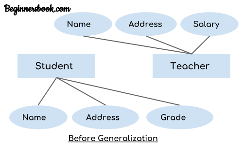
These two entities have two common attributes: Name and Address, we can make a generalized entity with these common attributes. Lets have a look at the ER model after generalization.
The ER diagram after generalization:
We have created a new generalized entity Person and this entity has the common attributes of both the entities. As you can see in the following ER diagram that after the generalization process the entities Student and Teacher only has the specialized attributes Grade and Salary respectively and their common attributes (Name & Address) are now associated with a new entity Person which is in the relationship with both the entities (Student & Teacher).
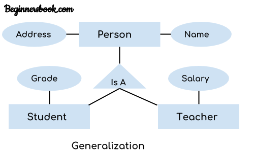
We have created a new generalized entity Person and this entity has the common attributes of both the entities. As you can see in the following ER diagram that after the generalization process the entities Student and Teacher only has the specialized attributes Grade and Salary respectively and their common attributes (Name & Address) are now associated with a new entity Person which is in the relationship with both the entities (Student & Teacher).
Note:
1. Generalization uses bottom-up approach where two or more lower level entities combine together to form a higher level new entity.
2. The new generalized entity can further combine together with lower level entity to create a further higher level generalized entity
1. Generalization uses bottom-up approach where two or more lower level entities combine together to form a higher level new entity.
2. The new generalized entity can further combine together with lower level entity to create a further higher level generalized entity
Difference between E-R Model and Relational Model in DBMS
E-R model and Relational model are two types of data models present in DBMS. Let’s have a brief look of them:
1. E-R Model :
E-R model stands for Entity Relationship model. ER Model is used to model the logical view of the system from data perspective which consists of these components: Entity, Entity Type, Entity Set.
E-R model stands for Entity Relationship model. ER Model is used to model the logical view of the system from data perspective which consists of these components: Entity, Entity Type, Entity Set.
An Entity may be an object with a physical existence – a particular person, car, house, or employee – or it may be an object with a conceptual existence – a company, a job, or a university course An Entity is an object of Entity Type and set of all entities is called as entity set. e.g.; E1 is an entity having Entity Type Student and set of all students is called Entity Set.
2. Relational model :
Relational Model was proposed by E.F. Codd to model data in the form of relations or tables. After designing the conceptual model of Database using ER diagram, we need to convert the conceptual model in the relational model which can be implemented using any RDMBS languages like Oracle SQL, MySQL etc.
Relational Model was proposed by E.F. Codd to model data in the form of relations or tables. After designing the conceptual model of Database using ER diagram, we need to convert the conceptual model in the relational model which can be implemented using any RDMBS languages like Oracle SQL, MySQL etc.
Consider a relation STUDENT with attributes ROLL_NO, NAME, ADDRESS, PHONE and AGE shown in Table 1.
STUDENT
| ROLL_NO | NAME | ADDRESS | PHONE | AGE |
| 1 | RAM | DELHI | 9455123451 | 18 |
| 2 | RAMESH | GURGAON | 9652431543 | 18 |
| 3 | SUJIT | ROHTAK | 9156253131 | 20 |
| 4 | SURESH | DELHI | 18 |
Let’s see the difference between ER model and relational model:
| S.NO. | ER MODEL | RELATIONAL MODEL |
|---|---|---|
| 1. | ER model is the high level or conceptual model. | It is the representational or implementation model. |
| 2. | It is used by people who don’t know how database is implemented. | It is used by programmers. |
| 3. | It represents collection of entities and describes relationship between them. | It represent data in the form of tables and describes relationship between them. |
| 4. | It consists of components like Entity, Entity Type, Entity Set. | It consists of components like domain, attributes, tuples. |
| 5. | It is easy to understand the relationship between entities. | It is less easy to derive the relationship between different tables. |
| 6. | It describes cardinality. | It does not describes cardinality |
DBMS Specialization
Specialization is a process in which an entity is divided into sub-entities. You can think of it as a reverse process of generalization, in generalization two entities combine together to form a new higher level entity. Specialization is a top-down process.
The idea behind Specialization is to find the subsets of entities that have few distinguish attributes. For example – Consider an entity employee which can be further classified as sub-entities Technician, Engineer & Accountant because these sub entities have some distinguish attributes.
Specialization Example
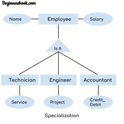
In the above diagram, we can see that we have a higher level entity “Employee” which we have divided in sub entities “Technician”, “Engineer” & “Accountant”. All of these are just an employee of a company, however their role is completely different and they have few different attributes. Just for the example, I have shown that Technician handles service requests, Engineer works on a project and Accountant handles the credit & debit details. All of these three employee types have few attributes common such as name & salary which we had left associated with the parent entity “Employee” as shown in the above diagram.
Aggregation –
An ER diagram is not capable of representing relationship between an entity and a relationship which may be required in some scenarios. In those cases, a relationship with its corresponding entities is aggregated into a higher level entity. For Example, Employee working for a project may require some machinery. So, REQUIRE relationship is needed between relationship WORKS_FOR and entity MACHINERY. Using aggregation, WORKS_FOR relationship with its entities EMPLOYEE and PROJECT is aggregated into single entity and relationship REQUIRE is created between aggregated entity and MACHINERY.
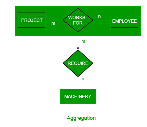
An ER diagram is not capable of representing relationship between an entity and a relationship which may be required in some scenarios. In those cases, a relationship with its corresponding entities is aggregated into a higher level entity. For Example, Employee working for a project may require some machinery. So, REQUIRE relationship is needed between relationship WORKS_FOR and entity MACHINERY. Using aggregation, WORKS_FOR relationship with its entities EMPLOYEE and PROJECT is aggregated into single entity and relationship REQUIRE is created between aggregated entity and MACHINERY.
No comments:
Post a Comment